06 Matrices of animal populations

Although the companion paper and the other raretrans vignettes focus on perennial plant data sets, the same Bayesian principles apply to animal populations. Small sample sizes compromise the estimation of survival and reproduction whenever the analyst believes that matrix entries should vary by age, sex, or environmental condition. In some cases there are no data at all for a particular combination of stage and environment, and the analysis must proceed using expert opinion—what Bayesians call prior beliefs.

Expressing those beliefs as probability distributions (rather than single point estimates) has two practical advantages. First, it forces the analyst to be explicit about how confident they are in each parameter. Second, it provides a principled way to propagate that uncertainty through derived quantities such as the asymptotic population growth rate $\lambda$ , the stable stage distribution, or extinction risk.

This vignette walks through a published Population Viability Analysis (PVA) for the endangered Florida Snail Kite and shows, step by step, how to re-express the original normal-distribution assumptions as Beta priors. The example does not use the raretrans functions directly because the published information is given as means and standard deviations rather than as raw transition counts. Nevertheless, the underlying logic—combining prior beliefs with data through conjugate Bayesian models—is exactly the same. A final section at the end shows how to connect this workflow back to raretrans when count data are available.

library(dplyr)
library(tidyr)
library(purrr)
library(tibble)
library(ggplot2)
library(popbio)
library(huxtable)

# Raymond's theme modifications
rlt_theme <- theme(axis.title.y = element_text(colour="grey20",size=15,face="bold"),
        axis.text.x = element_text(colour="grey20",size=15, face="bold"),
        axis.text.y = element_text(colour="grey20",size=15,face="bold"),  
        axis.title.x = element_text(colour="grey20",size=15,face="bold"))

Snail kites

Background

The Florida Snail Kite (Rostrhamus sociabilis plumbeus) is a wetland raptor that feeds almost exclusively on apple snails (Pomacea paludosa). Because snails are sensitive to water depth, periodic drought events in the Everglades create a direct link between hydrological management and kite demography. Stephen Beissinger (1995) developed a stage-based PVA to evaluate how the frequency of drought cycles affects the kite’s long-term viability. This study is a classic example of how expert opinion fills the gaps left by sparse field data.

Study design and data sources

Radio-telemetry and nest monitoring provided reasonably reliable survival and nest-success estimates for “high water” years, but data for “drought” and “lag” (recovery) years were far scarcer. Beissinger used a combination of field observations and expert judgement to assign parameter values for those environments. The model distinguished three age classes—fledgling, subadult, and adult—because small sample sizes precluded a finer age structure.

The table below (reproduced from Table 2 of Beissinger (1995)) summarises the vital rates used in the PVA. For each combination of environmental state and age class, means, standard deviations, and ranges are given for both nest success and annual survival. Beissinger sampled these parameters from normal distributions during the stochastic simulations.

b1995_table2 <- tribble(
  ~env_state, ~age_class, ~mean_ns, ~sd_ns, ~range_ns, ~prop_nesting, ~attempts, ~mean_s, ~sd_s, ~range_s,
  "", "", "Nesting success", "","", "", "", "Annual survival", "","",
  "Environmental state", "Age Class", "Mean", "SD","Range", "Proportion Nesting", 
  "Nesting attempts per year", "Mean", "SD", "Range",
  "Drought year", "Fledgling", "0.00", "0.00", "0.00-0.00", "0.00", "0.00", "0.50","0.10", "0.30-0.80",
  "", "Subadult", "0.03", "0.10", "0.00-0.25", "0.15", "1.00", "0.60", "0.10", "0.40-0.90",
  "", "Adult", "0.03", "0.10", "0.00-0.25", "0.15", "1.00", "0.60", "0.10", "0.40-0.90",
  "Lag year", "Fledgling", "0.00", "0.00", "0.00-0.00", "0.00", "0.00", "0.85","0.03", "0.75-0.92",
  "", "Subadult", "0.16", "0.10", "0.04-0.33", "0.15", "1.00", "0.90", "0.03", "0.80-0.95",
  "", "Adult",  "0.16", "0.10", "0.04-0.33", "0.80", "1.50", "0.90", "0.03", "0.80-0.95",
  "High year", "Fledgling", "0.00", "0.00", "0.00-0.00", "0.00", "0.00", "0.90","0.03", "0.75-0.92",
  "", "Subadult", "0.30", "0.10", "0.1-0.40", "0.25", "1.00", "0.95", "0.03", "0.85-0.98",
  "", "Adult", "0.30", "0.10", "0.1-0.40", "1.00", "2.20", "0.95", "0.03", "0.85-0.98")

huxtable(b1995_table2) %>% 
  set_colspan(row = 1, col = c(3,8), value = 3) %>% 
  theme_article(header_col = FALSE) %>% 
  set_width(0.9) %>% 
  set_col_width(c(0.15, 0.1, 0.075, 0.075, 0.1, 0.15, 0.15, 0.075, 0.075, 0.1)) %>% 
  set_position("left") %>% 
  set_bottom_border(row = 1, col = everywhere, value = 0) %>% 
  set_bottom_border(row = 2, col = everywhere, value = 1) %>% 
  set_caption("Snail kite vital rates from Beissinger (1995), Table 2.")

Snail kite vital rates from Beissinger (1995), Table 2.
		Nesting success					Annual survival
Environmental state	Age Class	Mean	SD	Range	Proportion Nesting	Nesting attempts per year	Mean	SD	Range
Drought year	Fledgling	0.00	0.00	0.00-0.00	0.00	0.00	0.50	0.10	0.30-0.80
	Subadult	0.03	0.10	0.00-0.25	0.15	1.00	0.60	0.10	0.40-0.90
	Adult	0.03	0.10	0.00-0.25	0.15	1.00	0.60	0.10	0.40-0.90
Lag year	Fledgling	0.00	0.00	0.00-0.00	0.00	0.00	0.85	0.03	0.75-0.92
	Subadult	0.16	0.10	0.04-0.33	0.15	1.00	0.90	0.03	0.80-0.95
	Adult	0.16	0.10	0.04-0.33	0.80	1.50	0.90	0.03	0.80-0.95
High year	Fledgling	0.00	0.00	0.00-0.00	0.00	0.00	0.90	0.03	0.75-0.92
	Subadult	0.30	0.10	0.1-0.40	0.25	1.00	0.95	0.03	0.85-0.98
	Adult	0.30	0.10	0.1-0.40	1.00	2.20	0.95	0.03	0.85-0.98

Survival values

Why a Beta distribution?

In a stage-structured matrix with $k$ possible fates (including death), survival probabilities form a multinomial, and the natural conjugate prior is a Dirichlet distribution (the approach used by raretrans). In this particular age-structured model, however, an individual of a given age can only survive to the next age class or die—exactly two possible outcomes. The Binomial likelihood paired with a $\text{Beta}(\alpha, \beta)$ prior is therefore sufficient.

The Beta distribution is bounded on $[0, 1]$ , making it appropriate for probabilities. Its two parameters $\alpha$ and $\beta$ can be interpreted as pseudo-counts: $\alpha$ “prior survivals” and $\beta$ “prior deaths”. Their sum $\alpha + \beta$ acts as an effective sample size that controls how concentrated the distribution is around its mean.

Moment matching: from mean and SD to $\alpha$ and $\beta$

The mean and variance of a $\text{Beta}(\alpha, \beta)$ distribution are:

$\mu = \frac{\alpha}{\alpha + \beta}, \qquad \sigma^2 = \frac{\alpha \beta}{\left(\alpha + \beta\right)^2\left(\alpha + \beta + 1\right)}$

Beissinger (1995) reports $\mu$ and $\sigma$ (Table 2). We can recover approximate $\alpha$ and $\beta$ by moment matching—equating the distribution’s theoretical moments to the observed summary statistics. Defining the auxiliary quantity $\nu$ :

$\begin{align*} \nu &= \frac{\mu\left(1-\mu\right)}{\sigma^2} \\ \alpha &= \nu\,\mu \\ \beta &= \left(1-\mu\right)\,\nu \end{align*}$

This conversion is valid as long as $\sigma^2 < \mu(1 - \mu)$ , which is satisfied for all entries in Beissinger’s Table 2. The code below performs this conversion and displays the resulting $\alpha$ and $\beta$ values.

kite_parms <- b1995_table2 %>% 
  slice(-(1:2)) %>% # remove top two rows
  separate(col = range_ns, into = c("min_ns","max_ns"), sep = "-") %>% 
  separate(col = range_s, into = c("min_s","max_s"), sep = "-") %>% 
  mutate(across(.cols = 3:12, .fns = as.numeric)) %>% # convert to numeric
  mutate(nu_ns = mean_ns * (1 - mean_ns) / sd_ns^2,
         alpha_ns = mean_ns * nu_ns,
         beta_ns = (1-mean_ns)*nu_ns,
         nu_s = mean_s * (1 - mean_s) / sd_s^2,
         alpha_s = mean_s * nu_s,
         beta_s = (1-mean_s)*nu_s) %>% 
  # set infinite vales to missing
  mutate(across(where(is.numeric), ~ifelse(is.nan(.x), NA_real_, .x))) 
kite_parms %>% 
  select(env_state, age_class, alpha_ns, beta_ns, alpha_s, beta_s) %>% 
  mutate(across(where(is.numeric), ~format(.x, digits = 2))) %>% 
  bind_rows(tibble(env_state = c("","Environmental State"),
                   age_class = c("", "Age Class"),
                   alpha_ns = c("Nest Success", "$\\alpha$"),
                   beta_ns = c("", "$\\beta$"),
                   alpha_s = c("Survival", "$\\alpha$"),
                   beta_s = c("", "$\\beta$")), .) %>% 
  mutate(across(.cols = 3:6, ~case_when(grepl("NA",.x) ~ " ", 
                                        TRUE ~ .x))) %>% 
#  filter(age_class != "Fledgling") %>% 
  hux() %>% 
  set_escape_contents(row = 2, col = 3:6, value = FALSE) %>% 
  theme_article(header_col = FALSE) %>% 
  set_na_string(value = " ") %>% 
  set_position("left") %>% 
  set_caption("Values of $\\alpha$ and $\\beta$ for each age class and 
              environmental state. Fledglings have zero probability of 
              nest success in all environmental states.")

Values of $\alpha$ and $\beta$ for each age class and environmental state. Fledglings have zero probability of nest success in all environmental states.
		Nest Success		Survival
Environmental State	Age Class	$\alpha$	$\beta$	$\alpha$	$\beta$
Drought year	Fledgling			12	12.5
	Subadult	0.087	2.8	14	9.6
	Adult	0.087	2.8	14	9.6
Lag year	Fledgling			120	21.3
	Subadult	2.150	11.3	90	10.0
	Adult	2.150	11.3	90	10.0
High year	Fledgling			90	10.0
	Subadult	6.300	14.7	50	2.6
	Adult	6.300	14.7	50	2.6

Interpreting the effective sample size

One of the key benefits of re-expressing beliefs as Beta parameters is transparency: the sum $\alpha + \beta$ is the effective sample size, so a reader can immediately see how much confidence the analyst has placed in each estimate.

Looking at the table above, nest-success estimates carry less confidence in drought and lag years than in high water years, consistent with what Beissinger (1995) states qualitatively. For survival, however, two patterns emerge that are inconsistent with Beissinger’s intended beliefs:

Within each environmental state, fledgling survival has a larger effective sample size than subadult or adult survival. This happens because fledgling survival is lower (mean $\approx 0.5$ – $0.9$ ), so $\mu(1-\mu)$ is larger relative to a fixed $\sigma^2$ .
High water year estimates appear less confident (smaller $n$ ) than lag year estimates, despite being based on the best data.

Both artifacts arise because Beissinger fixed the standard deviation at 0.03 or 0.10 regardless of the mean. For a normally distributed parameter, the mean and standard deviation are independent, so a fixed SD implies a fixed level of precision. For a Beta distribution, however, the variance depends on both the mean and the concentration. Fixing $\sigma$ while changing $\mu$ implicitly changes the effective sample size in counter-intuitive ways.

This observation has a practical lesson: when converting from a normal parameterisation to a Beta, it is worth checking whether the implied effective sample sizes are scientifically reasonable. If they are not, the analyst may want to specify $\alpha$ and $\beta$ directly rather than relying on moment matching.

pdf_seq <- seq(-0.2,1.2,0.001)
plot_colors <- RColorBrewer::brewer.pal(3, "RdYlBu")
kite_parms2 <- kite_parms %>% 
  mutate(env_state = rep(env_state[c(1,4,7)], each = 3),
         n_ns = alpha_ns + beta_ns,
         n_s = alpha_s + beta_s,
         lwr_ns = pbeta(min_ns, alpha_ns, beta_ns),
         upr_ns = pbeta(max_ns, alpha_ns, beta_ns),
         lwr_s = pbeta(min_s, alpha_s, beta_s),
         upr_s = pbeta(max_s, alpha_s, beta_s),
         plot_ns = map2(alpha_ns, beta_ns, ~tibble(x_ns = pdf_seq,
                                                   d_ns = dbeta(x_ns, .x, .y))),
         plot_ns_norm = map2(mean_ns, sd_ns, ~tibble(x_nsn = pdf_seq,
                                                     d_ns_norm = dnorm(x_nsn, .x, .y),
                                                     d_ns_tnorm = dnorm(x_nsn, .x, .y)/
                                                       pnorm(0, .x, .y, lower.tail = FALSE))),
         plot_s = map2(alpha_s, beta_s, ~tibble(x_s = pdf_seq,
                                                d_s = dbeta(x_s, .x, .y))),
         plot_s_norm = map2(mean_s, sd_s, ~tibble(x_sn = pdf_seq,
                                                  d_s_norm = dnorm(x_sn, .x, .y),
                                                  d_s_tnorm = dnorm(x_sn, .x, .y)/
                                                    pnorm(1, .x, .y))),
  ) %>% 
  unnest(cols = c("plot_ns", "plot_s", "plot_ns_norm","plot_s_norm"), 
         names_repair = "unique") %>% 
  mutate(env_state = factor(env_state, levels = c("Drought year","Lag year", "High year")),
         age_class = factor(age_class, levels = c("Fledgling", "Subadult", "Adult")))

ggplot(data = kite_parms2) + 
  geom_area(mapping = aes(x = x_s, y = d_s), alpha = 0.75, fill = plot_colors[1], color=plot_colors[1], size = 1) + 
  geom_area(mapping = aes(x = x_sn, y = d_s_tnorm), alpha = 0.75, fill = plot_colors[3], color = plot_colors[3], size = 1) +
  facet_grid(env_state~age_class, scales = "free_x") +
  scale_x_continuous(limits = c(0,1)) + 
  labs(x = "Annual survival", y = "Density")+
  theme_classic()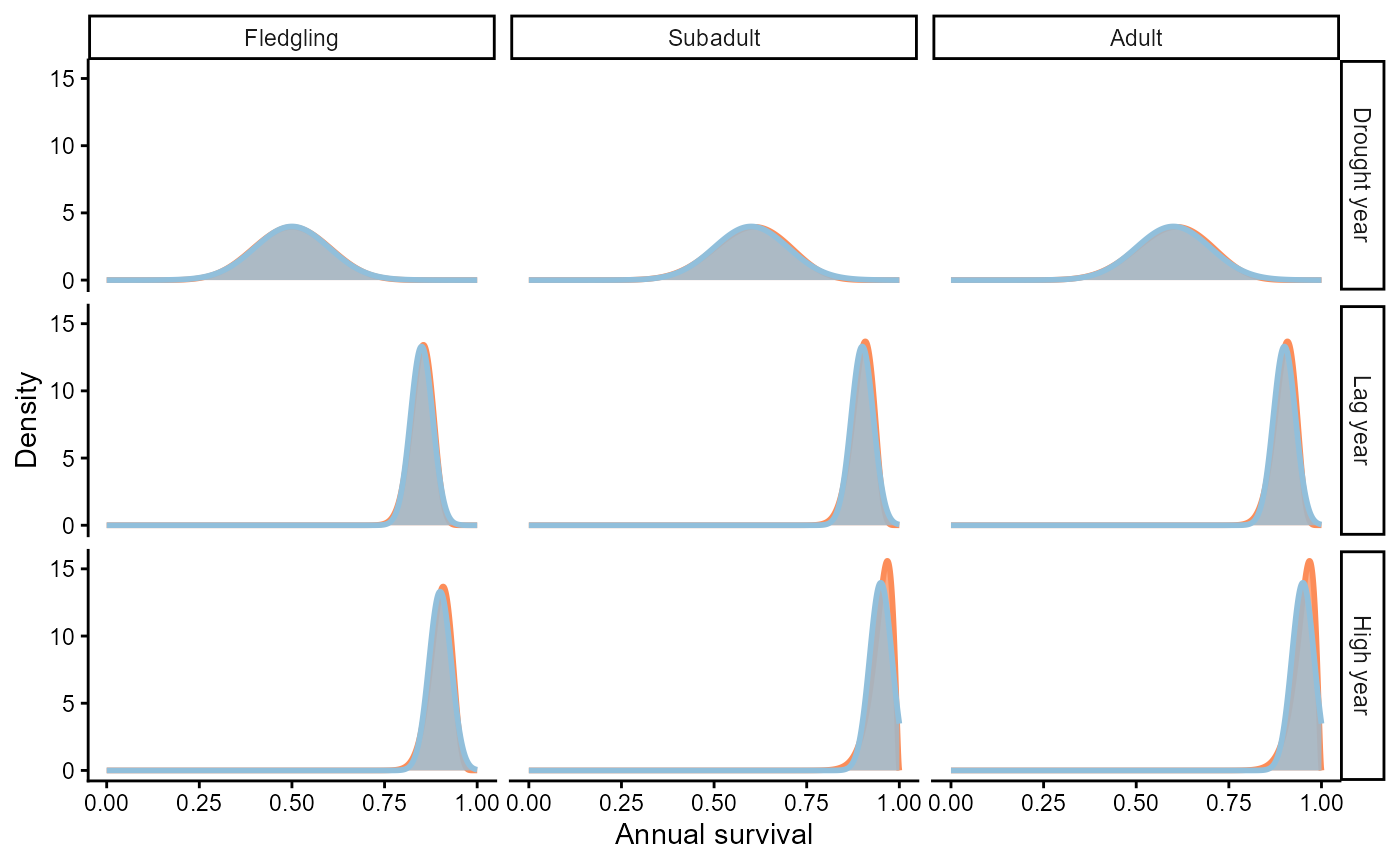

Probability distributions of annual survival by stage and environmental state. Beta distributions are red, truncated normal distributions are blue. Areas of overlap appear gray.

Comparing Beta and normal priors

The figure above overlays the Beta distribution (red) with the truncated normal (blue) used in the original PVA. Several points are worth noting:

For most stage–environment combinations the two distributions are nearly indistinguishable, confirming that the normal approximation works well when the mean is far from 0 or 1 and the standard deviation is small.
The approximation breaks down for subadult and adult survival in high water years, where mean survival is 0.95. Here the normal distribution assigns roughly 5% probability to values above 1.0—an impossible range for a probability. Beissinger (personal communication) dealt with this by rejecting inadmissible draws and resampling, effectively producing a truncated normal.
The truncation has little practical effect in this case, but in general it shifts the effective mean upward and can subtly bias simulation results.

The Beta distribution avoids these boundary issues entirely because it is defined on $[0, 1]$ by construction. This is one of the simplest arguments for preferring Beta (or Dirichlet) priors over normal distributions when modelling probabilities.

Reproductive rates

Components of reproduction

In the snail kite model, the fertility entry in column $j$ of the matrix is the product of four components:

$F_j = (\text{proportion nesting})_j \;\times\; (\text{nest attempts per year})_j \;\times\; (\text{nest success})_j \;\times\; (\text{young per successful nest})$

Beissinger (1995) treated all components except nest success as fixed values. For nest success—the probability that a nest produces at least one fledgling—means, standard deviations, and ranges were provided and sampled from normal distributions during the simulation.

Nest success as a Beta variable

Nest success is inherently a probability (bounded between 0 and 1), so a Beta distribution is the natural choice. Snyder et al. (1989) provide raw counts of successful and failed nests (their Table 3) that can be converted directly into Beta parameters: $\alpha$ = number of successful nests and $\beta$ = number of failed nests. This is more informative than the moment- matching approach because it uses the actual sample sizes rather than summary statistics.

Young per successful nest

Snyder et al. (1989) report an average of approximately 2 young per successful nest. Their Table 5 provides the actual distribution: 55, 110, and 47 nests produced 1, 2, or 3 young, respectively. This count data could be represented as a multinomial variable with a Dirichlet prior—exactly the approach that raretrans::fill_transitions() uses for transition probabilities. Although the mean number of young does not vary across environmental states, the sample sizes do, and this should be reflected in the confidence placed in each distribution. For simplicity, we use a fixed value of 2 young per successful nest in what follows.

Comparing prior sources

The code below builds Beta priors for nest success from the Snyder et al. (1989) counts and compares them with the moment-matched Beta and truncated normal distributions implied by Beissinger (1995).

repro_parms <- tribble(
  # prior_young is vector of nests with 1, 2, or 3 young. 
  # alpha_ns and beta_ns are the number of successful and unsuccessful nests
  ~env_state, ~age_class, ~prior_young, ~alpha_ns, ~beta_ns,
  "Drought year", "Subadult", c(1, 3, 1), 3, 91, 
  "Drought year", "Adult", c(1, 3, 1), 3, 91,
  "Lag year", "Subadult", c(6, 25, 8), 11, 58,
  "Lag year", "Adult", c(6, 25, 8), 11, 58,
  "High year", "Subadult", c(48, 82, 38), 100, 236,
  "High year", "Adult", c(48, 82, 38), 100, 236
)

repro_parms2 <- repro_parms %>% 
  mutate(n_ns = alpha_ns + beta_ns,
         plot_ns = map2(alpha_ns, beta_ns, ~tibble(x = pdf_seq,
                                                   d_ns = dbeta(x, .x, .y)))) %>% 
  unnest(plot_ns) %>% 
  mutate(env_state = factor(env_state, levels = c("Drought year","Lag year", "High year")),
         age_class = factor(age_class, levels = c("Fledgling", "Subadult", "Adult")))


ggplot(data = filter(repro_parms2, age_class != "Fledgling"),
       mapping = aes(x = x, y = d_ns)) + 
  geom_area(fill = plot_colors[2], alpha = 0.75, color=plot_colors[2], size = 1) + #Synder etal 1989
  geom_area(data = filter(kite_parms2, age_class != "Fledgling"), #Beissinger 1995
       mapping = aes(x = x_ns, y = d_ns), fill = plot_colors[1], alpha = 0.75, color=plot_colors[1], size = 1) + 
  geom_area(data = filter(kite_parms2, age_class != "Fledgling"), #Beissinger 1995
       mapping = aes(x = x_ns, y = d_ns_tnorm), fill = plot_colors[3], alpha = 0.75, color=plot_colors[3], size = 1) +   
  facet_grid(env_state~age_class, scales = "free_y") + 
  scale_x_continuous(limits = c(0,0.6)) +
#  scale_y_continuous(limits = c(0,30)) +
  labs(x = "Nest success", y = "Density") +
  rlt_theme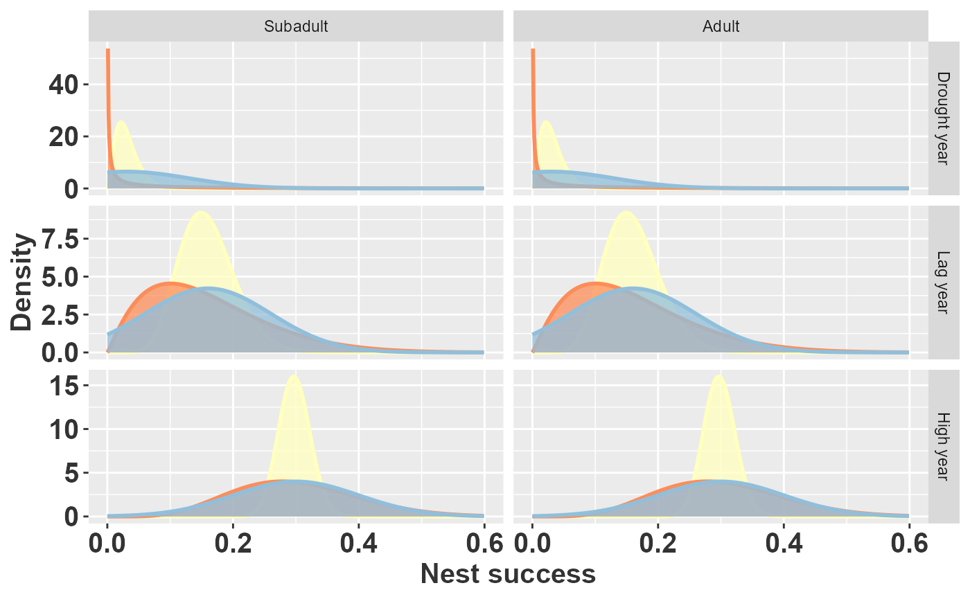

Prior beliefs about nest success using Beta distributions parameterized directly from Synder et al. (yellow, 1989), Beta distributions parameterized from Beissinger (red, 1995), and normal distributions from Beissinger (blue, 1995).

Interpretation

The figure reveals an important discrepancy. The yellow densities (Snyder et al. counts) are much narrower than the red densities (Beissinger moment-matched Beta), meaning the raw count data imply substantially more confidence in nest success than the summary statistics suggest. This may reflect a deliberate choice: because the other components of reproduction (proportion nesting, nest attempts, young per nest) were treated as known constants, Beissinger may have inflated the variance on nest success to partially compensate for the missing uncertainty in those components.

The blue densities (truncated normal from Beissinger) highlight a second issue. For drought years, where mean nest success is only 0.03, the normal distribution with $\sigma = 0.10$ assigns substantial probability to negative values. After truncation to $[0, 1]$ , the effective mean shifts upward to 0.092—roughly three times the intended value of 0.03. This systematic bias means the original PVA likely overestimated reproduction in drought years.

The Beta distribution avoids this problem entirely: it is defined on $[0, 1]$ , so no truncation or rejection sampling is needed, and the mean remains exactly where the analyst intends. This is a compelling practical reason to prefer Beta priors for probabilities, especially when the mean is close to the boundaries.

Building the matrices

Now that we have prior distributions for every vital rate, we can assemble them into a function that returns one realisation of the $3 \times 3$ age-structured projection matrix. Each call to this function draws survival probabilities from Beta distributions and combines them with nest success (also drawn from a Beta) and the fixed reproductive components to produce a complete matrix.

The matrix structure for the snail kite is:

$\mathbf{A} = \begin{pmatrix} 0 & F_2 & F_3 \\ s_1 & 0 & 0 \\ 0 & s_2 & s_3 \end{pmatrix}$

where $s_i$ is age-specific survival, $F_j$ is the fertility contribution from age class $j$ , and adults ( $s_3$ ) remain in the adult class indefinitely. Note that fledgling survival ( $s_1$ ) enters only through the fertility calculation (as a pre-breeding census correction), so the subdiagonal entry $A_{2,1}$ actually represents subadult survival.

# fix up parameter dataframes
surv_parms <- kite_parms %>% 
  mutate(env_state = rep(env_state[c(1,4,7)], each = 3)) 
repro_parms <- repro_parms %>% 
  left_join(select(surv_parms, env_state, age_class, prop_nesting, attempts))
snailkite_A <- function(e_state = "High year", 
                        s_parms = surv_parms,
                        r_parms = repro_parms){
  # assumes young per successful nest fixed at 2
  A <- matrix(0, nrow = 3, ncol = 3)
  surv_parms <- filter(s_parms, env_state == e_state)
  repro_parms <- filter(r_parms, env_state == e_state)
  surv <- rbeta(3, surv_parms$alpha_s, surv_parms$beta_s)
  A[2,1] <- surv[2]
  A[3,2] <- A[3,3] <- surv[3]
  ns <- rbeta(2, repro_parms$alpha_ns, repro_parms$beta_ns)
  A[1,2:3] <- repro_parms$prop_nesting * repro_parms$attempts * ns * 2 * surv[1]
  A
}
snailkite_A()
#>      [,1]  [,2]  [,3]
#> [1,] 0.00 0.140 1.308
#> [2,] 0.94 0.000 0.000
#> [3,] 0.00 0.995 0.995
snailkite_A("Drought year")
#>       [,1]    [,2]    [,3]
#> [1,] 0.000 0.00512 0.00498
#> [2,] 0.801 0.00000 0.00000
#> [3,] 0.000 0.62768 0.62768
snailkite_A("Lag year")
#>       [,1]   [,2]  [,3]
#> [1,] 0.000 0.0488 0.162
#> [2,] 0.876 0.0000 0.000
#> [3,] 0.000 0.9477 0.948

Propagating uncertainty to $\lambda$

With the matrix-generating function in hand, we can perform a Monte Carlo simulation: draw many matrices for each environmental state and compute the dominant eigenvalue $\lambda$ (asymptotic population growth rate) for each one. The resulting distribution of $\lambda$ values is a posterior predictive distribution that reflects all the uncertainty encoded in our priors.

A population is expected to grow when $\lambda > 1$ and decline when $\lambda < 1$ . By examining the proportion of simulated $\lambda$ values that fall below 1, we get an intuitive measure of extinction risk for each environmental state.

results <- tibble(
  e_state = factor(rep(c("Drought year", "Lag year", "High year"), each = 100),
                   levels = c("Drought year", "Lag year", "High year")),
  A = map(e_state, snailkite_A),
  lambda = map_dbl(A, lambda)
)
ggplot(data = results,
       mapping = aes(x = lambda)) + 
  geom_histogram(binwidth = 0.05) + 
  facet_wrap(~e_state) +
  rlt_theme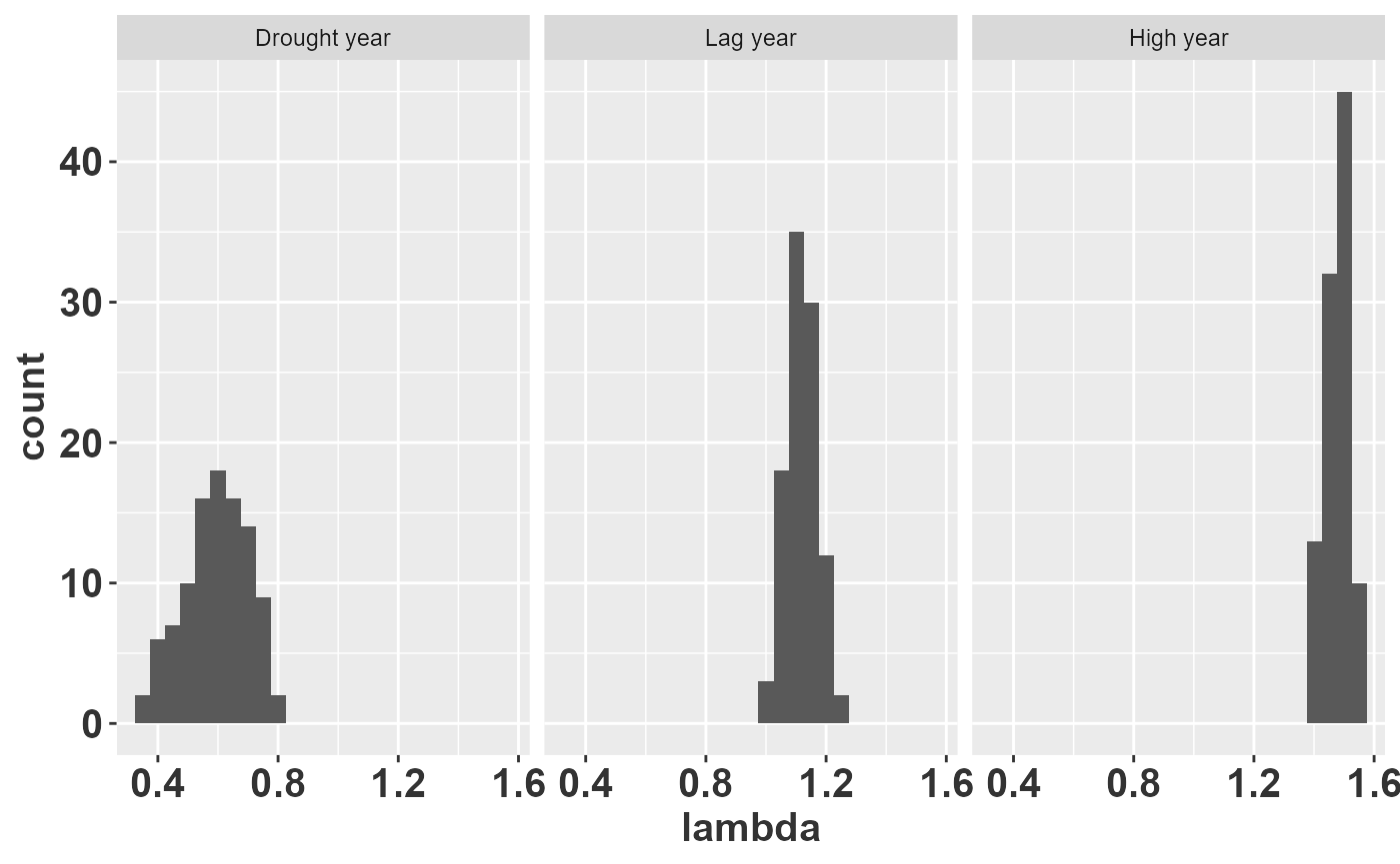

The histograms show that drought years produce $\lambda$ values well below 1 (population decline), high water years are consistently above 1 (population growth), and lag years fall near or slightly below 1. The spread of each histogram reflects parameter uncertainty: wider distributions indicate less confidence in the predicted growth rate. This kind of output is precisely what a PVA needs to assess the probability of decline under alternative management scenarios.

We could extend this further to reproduce the full extinction risk analysis in Beissinger (1995) by simulating sequences of environmental states and projecting the population forward in time.

Connection to `raretrans`

This vignette built Beta priors by hand because the published data were reported as means and standard deviations rather than as raw transition counts. When individual-level mark–recapture or census data are available—as in the orchid examples in the other vignettes—the raretrans package automates the entire workflow:

fill_transitions() combines observed fate counts with a Dirichlet prior (the multivariate generalisation of the Beta) to produce regularised transition probabilities. This is the direct analogue of the moment-matching step above, but using counts instead of summary statistics.
fill_fertility() does the same for reproduction using a Gamma–Poisson conjugate model.
sim_transitions() draws posterior matrices in a single call, replacing the custom snailkite_A() function we wrote above.
transition_CrI() and its companion plotting functions (plot_transition_CrI(), plot_transition_density()) produce the credible intervals and density visualisations that we computed manually for the kite.

The conceptual framework is identical in both cases: specify prior beliefs, update them with data, and propagate the resulting uncertainty to quantities of ecological interest. raretrans simply packages the most common version of this workflow—Dirichlet–multinomial transitions with count data—into a convenient set of functions that work with the standard TF list format used by popbio.

Literature cited

Beissinger, Steven R. 1995. “Modeling Extinction in Periodic Environments: Everglades Water Levels and Snail Kite Population Viability.” Ecological Applications 5 (3): 618–31. http://www.jstor.org/stable/1941971.

Snyder, Noel F. R., Steven R. Beissinger, and Roderick E. Chandler. 1989. “Reproduction and Demography of the Florida Everglade (Snail) Kite.” The Condor 91 (2): 300–316. http://www.jstor.org/stable/1368308.