02 Introduction to raretrans

knitr::opts_chunk$set(echo = TRUE, tidy = FALSE, collapse = TRUE, comment = "#>")
library(raretrans)

Overview

Matrix population models are a standard tool in ecology for projecting population dynamics and quantifying the contributions of survival, growth, and reproduction to population growth. A population projection matrix $\mathbf{A}$ is typically split into two components:

$\mathbf{T}$ — the transition matrix, whose columns describe the probabilities of surviving and moving between life-history stages (or staying in the same stage).
$\mathbf{F}$ — the fecundity matrix, whose entries describe the average number of offspring contributed to each stage by each adult stage.

The full model is $\mathbf{A} = \mathbf{T} + \mathbf{F}$ , and the asymptotic population growth rate $\lambda$ is the dominant eigenvalue of $\mathbf{A}$ .

Biased estimates from small samples

When populations are small or study periods are short, the observed transition frequencies produce two distinct types of biased estimates:

Structural zeros: biologically possible transitions that are never observed and appear as 0% in the data. These are rare events missed by chance — not truly impossible transitions.

Structural ones: transitions estimated at 100% survival, stasis, or mortality. For example, if all 3 observed juveniles survived, the data suggest 100% juvenile survival — a biologically implausible certainty caused entirely by small sample size.

Both are artefacts of insufficient data, and both distort the matrix:

A matrix with structural zeros may fail to be ergodic (some stages become unreachable) or reducible (some subsets of stages are disconnected).
A matrix with structural ones overestimates certainty in vital rates, producing a falsely precise and biologically unrealistic model.
In either case, the asymptotic growth rate $\lambda$ may be substantially biased.

raretrans addresses both problems by using Bayesian priors to regularise estimates, adding prior biological knowledge to the observed data so that all transitions receive a credible, non-extreme estimate.

The example population: Chamaedorea elegans

Throughout this vignette we use a published matrix for the understorey palm Chamaedorea elegans (parlour palm), compiled by Burns et al. (2013) and archived in the COMPADRE Plant Matrix Database (Salguero-Gómez et al. 2015). The population has three life-history stages:

Stage label	Description
`seed`	Propagule (seed)
`nonrep`	Non-reproductive individual (seedling/juvenile)
`rep`	Reproductive adult

The transition ( $\mathbf{T}$ ) and fecundity ( $\mathbf{F}$ ) matrices are entered directly below. This is the standard way to provide data to raretrans when you do not have individual-level observations.

# ── Transition matrix T ────────────────────────────────────────────────────────
# Each column must sum to ≤ 1 (the remainder is mortality).
# Rows = destination stage; Columns = source stage.
T_mat <- matrix(
  c(0.2368, 0.0000, 0.0000,   # seed  → seed, nonrep, rep
    0.0010, 0.0100, 0.0200,   # nonrep → seed, nonrep, rep
    0.0000, 0.1429, 0.1364),  # rep  → seed, nonrep, rep
  nrow = 3, ncol = 3, byrow = TRUE,
  dimnames = list(c("seed", "nonrep", "rep"),
                  c("seed", "nonrep", "rep"))
)

# ── Fecundity matrix F ─────────────────────────────────────────────────────────
# F[i,j] = average number of stage-i individuals produced by one stage-j parent.
F_mat <- matrix(
  c(0, 0, 1.9638,   # reproductive adults produce seeds
    0, 0, 8.3850,   # reproductive adults produce nonreproductive offspring
    0, 0, 0.0000),  # no fecundity contributions to the reproductive stage
  nrow = 3, ncol = 3, byrow = TRUE,
  dimnames = list(c("seed", "nonrep", "rep"),
                  c("seed", "nonrep", "rep"))
)

# ── Wrap in a named list — the format expected by raretrans ────────────────────
TF <- list(T = T_mat, F = F_mat)
TF
#> $T
#>          seed nonrep    rep
#> seed   0.2368 0.0000 0.0000
#> nonrep 0.0010 0.0100 0.0200
#> rep    0.0000 0.1429 0.1364
#> 
#> $F
#>        seed nonrep    rep
#> seed      0      0 1.9638
#> nonrep    0      0 8.3850
#> rep       0      0 0.0000

Each column of $\mathbf{T}$ describes one source stage. For example, the column seed tells us that in one time step a seed has:

a 23.7% chance of remaining a seed (seed → seed),
a 0.1% chance of germinating and becoming non-reproductive (seed → nonrep), and
the remaining ~76% chance of dying (not shown; implied by the column sum < 1).

The $\mathbf{F}$ matrix shows that only reproductive adults (rep) contribute offspring: each adult produces on average 1.96 seeds and 8.39 non-reproductive individuals per time step. These large fecundity values are typical for tropical palms that invest heavily in reproduction.

Providing the stage-population vector N

Many functions in raretrans require the starting number of individuals observed in each stage at the beginning of the census period. This vector $\mathbf{N}$ is used to convert the transition probabilities back to raw counts (because the Bayesian model works on counts, not proportions).

If you have individual-level data in a data frame you can use get_state_vector() to extract $\mathbf{N}$ automatically (see the onepopperiod vignette for a worked example). Here we supply it directly, using a hypothetical census of 80 seeds, 25 non-reproductive plants, and 12 reproductive adults.

N <- c(seed = 80, nonrep = 25, rep = 12)
N
#>   seed nonrep    rep 
#>     80     25     12

Part 1: Observed matrix and its limitations

Before adding any priors, let us examine the raw matrix.

# Dominant eigenvalue = asymptotic growth rate λ
A_obs <- TF$T + TF$F
lambda_obs <- Re(eigen(A_obs)$values[1])
cat("Observed lambda:", round(lambda_obs, 3), "\n")
#> Observed lambda: 1.171

Now look at the column sums of $\mathbf{T}$ :

colSums(TF$T)
#>   seed nonrep    rep 
#> 0.2378 0.1529 0.1564

The seed column sums to only 0.2378. The rest (0.7622) represents mortality of seeds. Importantly, the transition from seed to nonrep is 0.001 — very small and easily missed in a short study. In a small sample we might observe zero such transitions, leaving a structural zero in the data matrix even though we know germination happens.

Similarly, the nonrep → rep entry (0.1429) and the back-transition rep → nonrep (0.0200) could be missed in small populations. Conversely, if all observed individuals in a stage survived, the data would show a structural one (100% survival or stasis) — equally unreliable because it is driven by small sample size rather than biology. When either type of bias appears in real data, we need a principled way to incorporate our biological knowledge and regularise the estimates.

Part 2: Adding priors with `fill_transitions()`

Uniform (non-informative) prior

The simplest prior is the uniform Dirichlet prior. It adds a small equal weight to every possible fate. For a 3-stage system there are 4 fates per column (3 stages + death), so a uniform prior with weight 1 adds 0.25 to each fate count.

The prior matrix P has one more row than the transition matrix $\mathbf{T}$ : the extra row represents death.

# Uniform prior: equal weight to all fates (including death)
P_uniform <- matrix(0.25, nrow = 4, ncol = 3)
fill_transitions(TF, N, P = P_uniform)
#>             [,1]        [,2]       [,3]
#> [1,] 0.236962963 0.009615385 0.01923077
#> [2,] 0.004074074 0.019230769 0.03769231
#> [3,] 0.003086420 0.147019231 0.14513846

Compare with the original $\mathbf{T}$ :

TF$T
#>          seed nonrep    rep
#> seed   0.2368 0.0000 0.0000
#> nonrep 0.0010 0.0100 0.0200
#> rep    0.0000 0.1429 0.1364

The uniform prior has filled in all the zero entries, including the biologically impossible seed → rep transition. This is one weakness of a uniform prior: it does not distinguish between rare-but-possible transitions and impossible ones. This is an example and should NOT be used as a default prior in practice.

Informative (expert) prior

A better approach is to use an informative prior that reflects biological knowledge. The prior matrix still has 4 rows (3 stages + death), and ideally each column sums to 1 so that the weight is easy to interpret.

For C. elegans we specify:

Seeds have a high chance of dying (0.70), a moderate chance of staying as a seed (0.25), and a small chance of germinating to non-reproductive (0.05); the direct jump to reproductive is impossible (0.00).
Non-reproductive plants mostly stay non-reproductive (0.55) or die (0.25); they can grow to reproductive (0.15) but very rarely revert to seed (0.05).
Reproductive adults mostly stay reproductive (0.70) or die (0.10); they can revert to non-reproductive (0.15) or, very rarely, to seed (0.05).

P_info <- matrix(
  c(0.25, 0.05, 0.00,   # → seed
    0.05, 0.55, 0.15,   # → nonrep
    0.00, 0.15, 0.70,   # → rep
    0.70, 0.25, 0.15),  # → dead
  nrow = 4, ncol = 3, byrow = TRUE
)
# Verify columns sum to 1
colSums(P_info)
#> [1] 1 1 1

Now apply this prior with the default weight of 1 (equivalent to adding 1 individual’s worth of prior “observations”):

T_posterior <- fill_transitions(TF, N, P = P_info)
T_posterior
#>             [,1]        [,2]      [,3]
#> [1,] 0.236962963 0.001923077 0.0000000
#> [2,] 0.001604938 0.030769231 0.0300000
#> [3,] 0.000000000 0.143173077 0.1797538

The informative prior fills in the rare transitions without creating the impossible seed → rep entry (which stays at 0 because we set that prior entry to 0).

Adjusting prior weight

The priorweight argument controls how strongly the prior influences the posterior. A weight of 1 (the default) means the prior counts as 1 individual. Setting priorweight = 0.5 halves that influence:

fill_transitions(TF, N, P = P_info, priorweight = 0.5)
#>            [,1]       [,2]       [,3]
#> [1,] 0.24120000 0.01666667 0.00000000
#> [2,] 0.01733333 0.19000000 0.06333333
#> [3,] 0.00000000 0.14526667 0.32426667

With priorweight = 0.5 and $N = 25$ non-reproductive plants observed, the effective prior sample size for that column is $0.5 \times 25 = 12.5$ individuals, still less than the data. This is the recommended approach: the prior sample size should be smaller than the observed sample size so that the data dominate the posterior.

Part 3: Adding priors for fecundity with `fill_fertility()`

The fecundity prior follows a Gamma-Poisson (negative binomial) model. We specify two matrices, alpha and beta, whose entries are the shape and rate parameters of the Gamma prior on the Poisson rate. Use NA for entries that represent stages that cannot reproduce or fates that do not arise from reproduction.

# alpha = prior "offspring counts"; beta = prior "adult counts"
# Only the (seed, rep) and (nonrep, rep) entries are reproductive
alpha <- matrix(
  c(NA, NA, 1e-5,
    NA, NA, 1e-5,
    NA, NA, NA),
  nrow = 3, ncol = 3, byrow = TRUE
)
beta <- matrix(
  c(NA, NA, 1e-5,
    NA, NA, 1e-5,
    NA, NA, NA),
  nrow = 3, ncol = 3, byrow = TRUE
)

F_posterior <- fill_fertility(TF, N, alpha = alpha, beta = beta)
F_posterior
#>        seed nonrep      rep
#> seed      0      0 1.963799
#> nonrep    0      0 8.384994
#> rep       0      0 0.000000

The tiny values of alpha and beta (1e-5) produce a nearly non-informative prior: the posterior fecundity is almost identical to the observed fecundity because the data completely dominate. This is the correct behaviour when you have no prior information about fecundity.

Combined posterior matrix

posterior <- list(
  T = fill_transitions(TF, N, P = P_info),
  F = fill_fertility(TF, N, alpha = alpha, beta = beta)
)
posterior
#> $T
#>             [,1]        [,2]      [,3]
#> [1,] 0.236962963 0.001923077 0.0000000
#> [2,] 0.001604938 0.030769231 0.0300000
#> [3,] 0.000000000 0.143173077 0.1797538
#> 
#> $F
#>        seed nonrep      rep
#> seed      0      0 1.963799
#> nonrep    0      0 8.384994
#> rep       0      0 0.000000

# Asymptotic growth rate of the posterior matrix
lambda_post <- Re(eigen(posterior$T + posterior$F)$values[1])
cat("Posterior lambda:", round(lambda_post, 3), "\n")
#> Posterior lambda: 1.206
cat("Observed lambda:", round(lambda_obs, 3), "\n")
#> Observed lambda: 1.171

The posterior $\lambda$ is slightly different from the observed $\lambda$ because the prior redistributes a small amount of probability mass from the observed transitions to the rare ones.

Part 4: Other return types

Both fill_transitions() and fill_fertility() accept a returnType argument for accessing different representations of the posterior.

Augmented fate matrix (TN)

Setting returnType = "TN" returns the augmented fate matrix — the raw Dirichlet posterior counts (not divided by column sums). The extra bottom row gives the posterior count for the death fate.

TN <- fill_transitions(TF, N, P = P_info, returnType = "TN")
TN
#>        [,1]    [,2]    [,3]
#> [1,] 19.194  0.0500  0.0000
#> [2,]  0.130  0.8000  0.3900
#> [3,]  0.000  3.7225  2.3368
#> [4,] 61.676 21.4275 10.2732

This is useful for simulation (see Part 5) and for computing credible intervals directly (see Part 6).

Full projection matrix A

Setting returnType = "A" returns $\mathbf{T} + \mathbf{F}$ directly:

fill_transitions(TF, N, P = P_info, returnType = "A")
#>               seed      nonrep       rep
#> seed   0.236962963 0.001923077 1.9638000
#> nonrep 0.001604938 0.030769231 8.4150000
#> rep    0.000000000 0.143173077 0.1797538

Alpha and beta vectors (fertility)

Setting returnType = "ab" in fill_fertility() returns the posterior Gamma parameters:

fill_fertility(TF, N, alpha = alpha, beta = beta, returnType = "ab")
#> $alpha
#>        seed nonrep       rep
#> seed     NA     NA  23.56561
#> nonrep   NA     NA 100.62001
#> rep      NA     NA        NA
#> 
#> $beta
#>      [,1] [,2]     [,3]
#> [1,]   NA   NA 12.00001
#> [2,]   NA   NA 12.00001
#> [3,]   NA   NA       NA

Part 5: Simulating matrices and credible intervals on $\lambda$

Point estimates of $\lambda$ do not convey uncertainty. To obtain a credible interval on the asymptotic growth rate we simulate many matrices from the posterior distribution using sim_transitions().

set.seed(20240301)  # for reproducibility

# Simulate 1000 projection matrices from the posterior
sims <- sim_transitions(TF, N,
                        P     = P_info,
                        alpha = alpha,
                        beta  = beta,
                        priorweight = 0.5,
                        samples = 1000)

# Extract λ from each simulated matrix
lambdas <- sapply(sims, function(mat) Re(eigen(mat)$values[1]))

# Summarise
cat("Posterior median λ:", round(median(lambdas), 3), "\n")
#> Posterior median λ: 1.009
cat("95% credible interval: [",
    round(quantile(lambdas, 0.025), 3), ",",
    round(quantile(lambdas, 0.975), 3), "]\n")
#> 95% credible interval: [ 0.729 , 1.338 ]
cat("P(λ > 1):", round(mean(lambdas > 1), 3), "\n")
#> P(λ > 1): 0.516

# Plot
hist(lambdas,
     breaks = 30,
     main   = expression("Posterior distribution of " * lambda),
     xlab   = expression(lambda),
     col    = "steelblue", border = "white")
abline(v = 1, lty = 2, lwd = 2, col = "firebrick")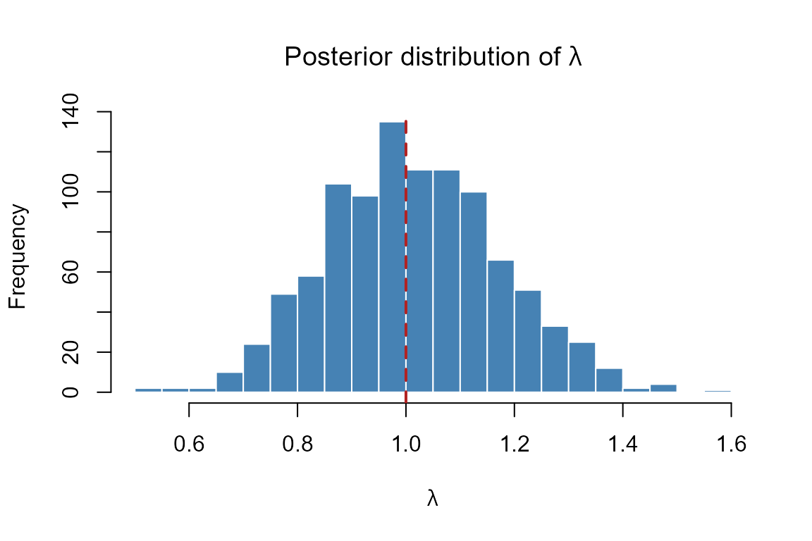

Posterior distribution of the asymptotic growth rate λ for Chamaedorea elegans. The dashed vertical line marks λ = 1 (stable population). Values to the right indicate growth; values to the left indicate decline.

The histogram shows the full posterior uncertainty about $\lambda$ . P(λ > 1) is the posterior probability that the population is growing — a more informative summary than a point estimate alone.

Part 6: Credible intervals on individual transition probabilities

Computing credible intervals with `transition_CrI()`

transition_CrI() computes the marginal posterior beta credible intervals for every entry in $\mathbf{T}$ , including the probability of dying. It returns a tidy data frame with one row per source–destination pair.

cri <- transition_CrI(TF, N,
                      P           = P_info,
                      priorweight = 0.5,
                      ci          = 0.95,
                      stage_names = c("seed", "nonrep", "rep"))
cri
#>    from_stage to_stage       mean        lower      upper
#> 1        seed     seed 0.24120000 1.692728e-01 0.32129406
#> 2        seed   nonrep 0.01733333 2.256578e-03 0.04705808
#> 3        seed      rep 0.00000000 0.000000e+00 0.00000000
#> 4        seed     dead 0.74146667 6.598519e-01 0.81546034
#> 5      nonrep     seed 0.01666667 6.264931e-05 0.07442516
#> 6      nonrep   nonrep 0.19000000 8.308126e-02 0.32809985
#> 7      nonrep      rep 0.14526667 5.337170e-02 0.27271819
#> 8      nonrep     dead 0.64806667 4.907560e-01 0.79041606
#> 9         rep     seed 0.00000000 0.000000e+00 0.00000000
#> 10        rep   nonrep 0.06333333 2.506019e-03 0.20938896
#> 11        rep      rep 0.32426667 1.354970e-01 0.54994310
#> 12        rep     dead 0.61240000 3.845731e-01 0.81658085

Each row gives the posterior mean transition probability and its 95% symmetric credible interval. The dead rows summarise the probability of mortality from each source stage.

Visualising credible intervals with `plot_transition_CrI()`

plot_transition_CrI(cri)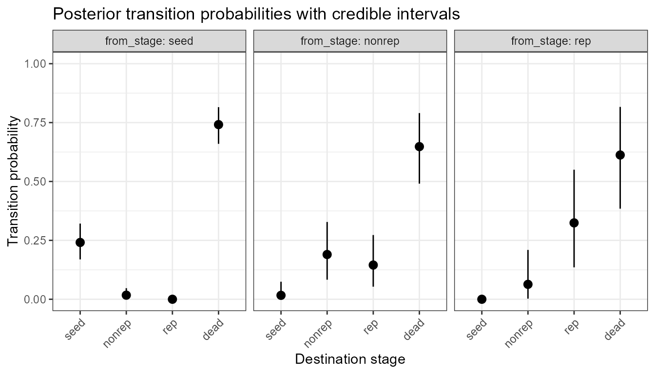

Posterior mean transition probabilities (points) and 95% credible intervals (lines) for Chamaedorea elegans. Each panel shows the fate distribution from one source stage.

You can hide the death fate if you prefer to focus on the living stages:

plot_transition_CrI(cri, include_dead = FALSE)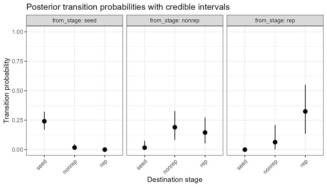

As above but excluding the dead fate.

Notice that the credible intervals for the seed → nonrep transition are very wide, reflecting the fact that this germination event is rarely observed (only 0.1% per time step in this matrix). The prior provides a small regularising signal but the data are sparse, so uncertainty is high.

Visualising the full posterior density with `plot_transition_density()`

plot_transition_density() arranges the full marginal posterior beta density for every transition as a matrix of panels, mirroring the layout of $\mathbf{T}$ . Each column corresponds to a source stage and each row to a destination stage. The shaded region is the 95% credible interval.

plot_transition_density(TF, N,
                        P           = P_info,
                        priorweight = 0.5,
                        stage_names = c("seed", "nonrep", "rep"))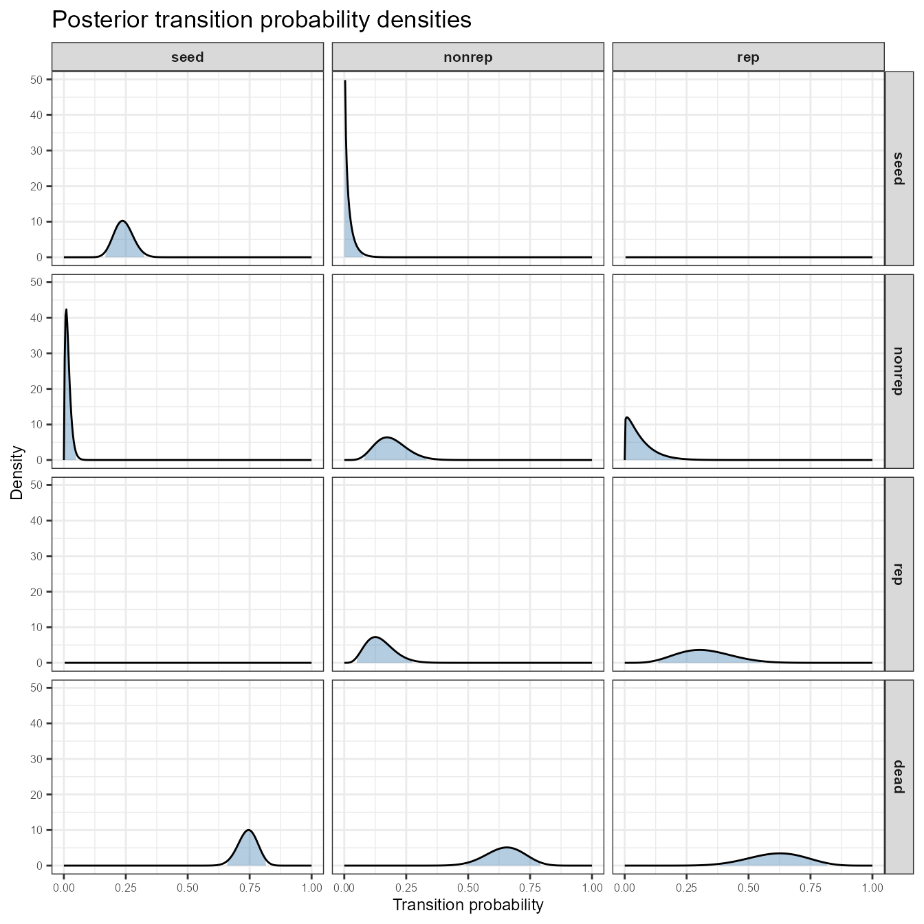

Posterior beta density for each transition in the C. elegans matrix. Columns = source stage (from); rows = destination stage (to). Shaded region = 95% credible interval. Zero-probability transitions show a degenerate spike at 0.

Panels on the main diagonal (e.g., seed → seed, rep → rep) tend to have well-constrained distributions because stasis is commonly observed. Off-diagonal transitions that are biologically rare show broad, flat densities — exactly where the prior matters most.

Excluding the death row gives a tighter layout focused on the living stages:

plot_transition_density(TF, N,
                        P             = P_info,
                        priorweight   = 0.5,
                        stage_names   = c("seed", "nonrep", "rep"),
                        include_dead  = FALSE)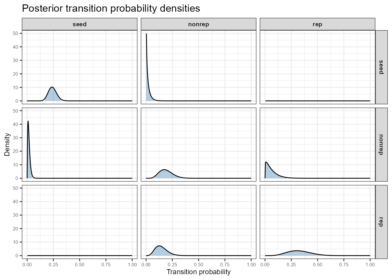

As above but excluding the dead fate row.

Summary

This vignette introduced the core workflow of raretrans:

Define your transition matrix $\mathbf{T}$ and fecundity matrix $\mathbf{F}$ , either from a data frame (using popbio::projection.matrix() and get_state_vector()) or by entering them directly.
Specify a prior matrix P that encodes biological knowledge about which transitions are possible and how likely they are. Prefer informative priors over the uniform default when you have relevant expertise.
Regularise estimates using fill_transitions() and fill_fertility() to correct structural zeros, structural ones, and other small-sample biases.
Simulate many matrices from the posterior with sim_transitions() to obtain a credible interval on $\lambda$ .
Visualise transition-level uncertainty with transition_CrI(), plot_transition_CrI(), and plot_transition_density().

For a worked example that starts from individual-level field observations see vignette("onepopperiod").

References

Burns, J., Blomberg, S., Crone, E., Ehrlén, J., Knight, T., Pichancourt, J.-B.,, Ramula, S., Wardle, G., & Buckley, Y. (2010). Empirical tests of life-history, evolution theory using phylogenetic analysis of plant demography., Journal of Ecology, 98(2), 334–344., https://doi.org/10.1111/j.1365-2745.2009.01634.x

Salguero-Gómez, R., Jones, O. R., Archer, C. R., Buckley, Y. M., Che-Castaldo, J., Caswell, H., …, & Vaupel, J. W. (2015). The COMPADRE Plant Matrix Database: an open online repository for plant demography. Journal of Ecology, 103, 202–218. https://doi.org/10.1111/1365-2745.12334

Tremblay, R. L., Tyre, A. J., Pérez, M.-E., & Ackerman, J. D. (2021). Population projections from holey matrices: Using prior information to estimate rare transition events. Ecological Modelling, 447, 109526. https://doi.org/10.1016/j.ecolmodel.2021.109526