01 Quick start: credible intervals for transition probabilities

What this vignette shows

This is a minimal worked example of the two most important functions in raretrans:

transition_CrI() — compute Bayesian credible intervals for every transition probability in a stage-structured matrix
plot_transition_CrI() — visualise those intervals

If you are new to Bayesian statistics, beta distributions, or Dirichlet priors, see the vignette Credible intervals for transition probabilities: Cypripedium calceolus (vignette("credible_intervals")), which explains those concepts in detail.

The data

We use a single transition period from population 231 of Lepanthes eltoroensis, a rare Puerto Rican orchid monitored annually. The data are included in raretrans as L_elto (see ?L_elto).

The population has three stages:

Code	Stage
`p`	Proto-adult
`j`	Juvenile
`a`	Adult

Stage m (missing next year) is treated as death.

From year 6 of population 231 we observed:

# Observed transitions (from -> to): n individuals
# a -> a : 18    j -> a : 2    p -> j : 1
# j -> j : 13    p -> p : 8    p -> m : 2  (died)
#
# No deaths observed in adults or juveniles — a classic holey matrix!
# raretrans handles this by placing prior weight on the dead fate.

Build the input matrices

raretrans needs a TF list with two matrices (T for transitions, F for fertility) and a vector N of observed individuals per stage.

library(raretrans)

stage_names <- c("proto", "juvenile", "adult")

# Transition matrix T (column = source stage, row = destination stage)
# Columns must be in the same order as stage_names
T_mat <- matrix(
  c(8,  0,  0,   # proto  -> proto, juvenile, adult
    1, 13,  0,   # juvenile -> proto, juvenile, adult
    0,  2, 18),  # adult  -> proto, juvenile, adult
  nrow = 3, ncol = 3, byrow = TRUE,
  dimnames = list(stage_names, stage_names)
)

# Fertility matrix F (no sexual reproduction observed this period)
F_mat <- matrix(0, nrow = 3, ncol = 3,
                dimnames = list(stage_names, stage_names))

TF <- list(T = T_mat, F = F_mat)

# Observed number of individuals at start of period (column sums of T + deaths)
N <- c(proto = 11, juvenile = 15, adult = 18)

T_mat
#>          proto juvenile adult
#> proto        8        0     0
#> juvenile     1       13     0
#> adult        0        2    18

Note that adults and juveniles have no observed deaths — their columns sum to less than N only because of transitions to other stages, not mortality. This is the holey matrix problem: a naive estimate would give survival probability = 1.0, which is biologically impossible.

Compute credible intervals

cri <- transition_CrI(TF, N, stage_names = stage_names)
#> Warning in stats::qbeta(alpha_lower, a, b): NaNs produced
#> Warning in stats::qbeta(alpha_upper, a, b): NaNs produced
#> Warning in stats::qbeta(alpha_lower, a, b): NaNs produced
#> Warning in stats::qbeta(alpha_upper, a, b): NaNs produced
#> Warning in stats::qbeta(alpha_lower, a, b): NaNs produced
#> Warning in stats::qbeta(alpha_upper, a, b): NaNs produced
cri
#>    from_stage to_stage         mean        lower      upper
#> 1       proto    proto   7.35416667          NaN        NaN
#> 2       proto juvenile   0.93750000 7.543166e-01 0.99941091
#> 3       proto    adult   0.02083333 2.317192e-08 0.13998339
#> 4       proto     dead  -7.31250000          NaN        NaN
#> 5    juvenile    proto   0.01562500 1.714579e-08 0.10560360
#> 6    juvenile juvenile  12.20312500          NaN        NaN
#> 7    juvenile    adult   1.89062500          NaN        NaN
#> 8    juvenile     dead -13.10937500          NaN        NaN
#> 9       adult    proto   0.01315789 1.434719e-08 0.08916703
#> 10      adult juvenile   0.01315789 1.434719e-08 0.08916703
#> 11      adult    adult  17.06578947          NaN        NaN
#> 12      adult     dead -16.09210526          NaN        NaN

Even though no adult deaths were observed, transition_CrI() returns a non-zero credible interval for the dead fate of adults and juveniles. The prior places a small but non-zero weight on mortality, producing biologically realistic estimates.

Visualise

Including the dead fate

plot_transition_CrI(cri,
                    title = "Lepanthes eltoroensis — population 231, year 6")
#> Warning: Removed 7 rows containing missing values or values outside the scale range
#> (`geom_pointrange()`).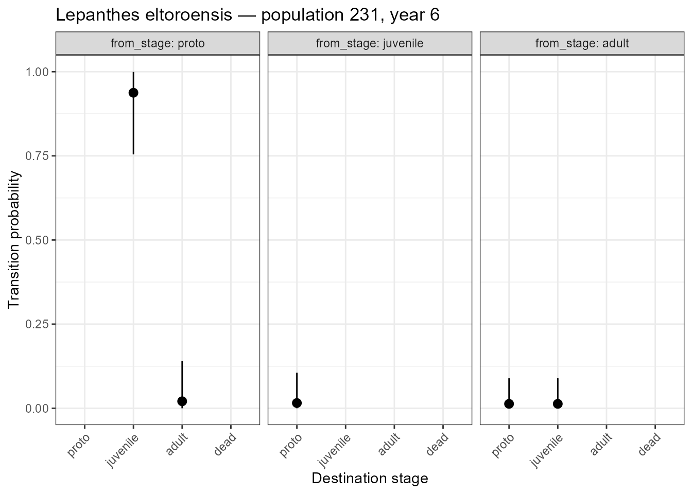

Posterior transition probabilities with 95% credible intervals. Note the non-zero dead fate for adults and juveniles despite zero observed deaths.

The wide credible intervals for the dead fate of adults and juveniles reflect genuine uncertainty — we know mortality must be possible, but we have no direct observations to estimate its rate precisely.

Excluding the dead fate

plot_transition_CrI(cri,
                    include_dead = FALSE,
                    title = "Lepanthes eltoroensis — survival transitions only")
#> Warning: Removed 4 rows containing missing values or values outside the scale range
#> (`geom_pointrange()`).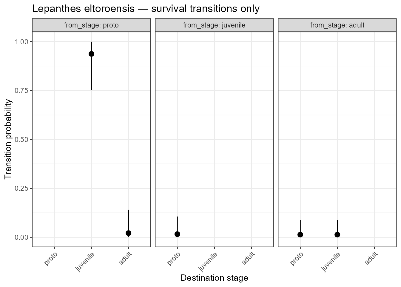

Posterior transition probabilities for survival transitions only.

Next steps

Topic	Vignette
Full posterior density plots	`vignette("credible_intervals")`
Effect of prior weight	`vignette("credible_intervals")`
Multi-period analysis	`vignette("onepopperiod")`
Prior choice and Bayesian background	`vignette("transition_priors")`

Reference

Tremblay, R. L., Tyre, A. J., Pérez, M.-E., & Ackerman, J. D. (2021). Population projections from holey matrices: Using prior information to estimate rare transition events. Ecological Modelling, 447, 109526. https://doi.org/10.1016/j.ecolmodel.2021.109526

Raymond Tremblay

2026-04-11